Singleton in fencing control protocol

The problem of singleton formation in fencing control is similar to the local minimum point in Artificial Potential Fields (APFs). This problem is discussed in Chen 2019 automatica¹ and our IJRNC work. The post is written to show some thinking when we investigate this problem.

1. Problem Description#

1.1 System Model#

• $N$ autonomous vehicles ($N \geq 3$), each vehicle’s position is $x_i = [x_{1,i}, x_{2,i}]^\top \in \mathbb{R}^2$
• Kinematic model: $\dot{x}_i(t) = u_i(t)$, where $u_i$ is the control input to be designed
• Designated target position: $x_o \in \mathbb{R}^2$
• $\text{co}(x)$ denotes the convex hull of vehicle positions
• $P_{x_o}(x) = \min_{s \in \text{co}(x)} \|x_o - s\|$: distance from the target to the convex hull
• $\text{area}(x)$: area of the convex hull (Lebesgue measure)

1.2 Control Objectives#

Design the controller $u_i$ such that the closed-loop system satisfies the following three properties:

Note: (P1) has two implications: (a) there exists a desired trajectory $x^*(t)$ such that the target lies within the convex hull of $x^*(t)$ at all times; (b) the actual trajectory asymptotically converges to $x^*(t)$.

1.3 Neighbor Definition#

The geographic neighbor set of vehicle $i$:

where $\mu > d > 0$ is the sensing range. The neighbor relation is symmetric, so the underlying graph is undirected.

2. Control Algorithm#

2.1 Controller Structure (Equation 2)#

The control input $u_i^o$ for each vehicle $i$ consists of three functional components:

where $x_{ij} = x_i - x_j$, and $R$ is the $90^\circ$ counterclockwise rotation matrix.

2.2 Detailed Description of Each Component#

(a) Attractive Component#

• Function: Drives each vehicle toward the target position
• Parameter: $k$ is the attraction gain

(b) Repulsive Component#

• Function: Avoids collisions between adjacent vehicles
• Properties of function $\alpha(s)$:
  • Domain: $(d, \infty) \to [0, \infty)$, continuous
  • $\alpha(s) = 0,\ \forall s \in [\mu, \infty)$ — no repulsive force beyond the sensing range
  • $\lim_{s \to d^+} \alpha(s) = \infty$ — repulsive force increases sharply as distance approaches $d$
• Physical meaning: When two vehicles are closer than $\mu$, a repulsive force arises along the line connecting them, increasing as the distance decreases

(c) Rotation Component#

• Function: When vehicles and the target are nearly collinear, generates a lateral rotational force to break the singleton straight-line formation
• Definition of $\beta$:

where:

• $\angle(x_{io}, x_{jo}) = \arccos\left(\frac{x_{io} \cdot x_{jo}}{\|x_{io}\|\|x_{jo}\|}\right) \in [0, \pi]$: the angle subtended by vehicles $i$ and $j$ as viewed from the target

• $\delta \in [0, \pi/2)$: angle threshold

• $\epsilon > 0$: rotation strength

• By convention, $\angle(0, a) = \angle(a, 0) = \pi$

• Activation condition: Activates when $\angle(x_{io}, x_{jo}) < \delta$, i.e., when the angle between the two vehicles as seen from the target is very small (vehicles and target are nearly collinear)

• Physical meaning: $R$ rotates the force direction by $90^\circ$, prompting the vehicle to “turn away” from the collinear configuration

3. Main Theoretical Results#

3.1 Theorem Statement (Theorem 2.1)#

For system (1) with control input $u_i = u_i^o$ (Equation 2), when $N > 3$, the target fencing problem is solved in the sense of (P1), (P2), and (P3), provided that:

• The vehicles are initially collision-free: $\|x_i(0) - x_j(0)\| > d,\ i \neq j$

Furthermore, if the control input is subject to exponentially decaying perturbations $e_i(t)$ (satisfying $\lim_{t \to \infty} e_i(t) = 0$), i.e., $u_i = u_i^o + e_i$, the conclusion still holds.

3.2 Proof Sketch#

(P1) Proof of Target Fencing#

1. The centroid of the vehicles $\bar{x} = \frac{1}{N}\sum_{i \in \mathbb{N}} x_i$ satisfies:

where $\bar{e} = \frac{1}{N}\sum_{i} e_i$. The derivation exploits the symmetry of the neighbor relation ($i \in \mathcal{N}_j \Leftrightarrow j \in \mathcal{N}_i$), $x_{ij} = -x_{ji}$, and $\beta(x_i, x_j, x_o) = \beta(x_j, x_i, x_o)$.

2. Since $\bar{e}(t) \to 0$ exponentially, the linear system drives $\bar{x}(t) \to x_o$.

3. The centroid always lies within the convex hull ($\bar{x} \in \text{co}(x)$), hence the target enters the convex hull: $P_{x_o}(x(t)) \to 0$.

(P2) Proof of Collision Avoidance#

1. Construct a Lyapunov potential function:

2. Compute its time derivative along the trajectory, yielding:

where $\|\psi_i\| \leq (N-1)\epsilon\delta$.

3. Integrating gives:

Since $\int \alpha(s)\,ds$ diverges as $s \to d^+$, it follows that $\|x_{ij}(t)\| > d$ holds at all times.

(P3) Proof of No Singleton Formation (Proof by Contradiction)#

1. Assume $\mathcal{S}$ is an invariant set, i.e., the vehicles remain collinear with the target at all times.
2. Due to collision avoidance, the ordering of vehicles along the line is invariant. Denote the two extreme vehicles as $\bar{h}$ and $\ell$.
3. From (P1), the centroid converges to the target, so there exists a time $T$ after which the target lies between the two extreme vehicles.
4. Analyze the velocities of the extreme vehicles: when an extreme vehicle has no neighbors, its velocity relative to the other extreme vehicle exceeds $k(N-1)d/2$, inevitably leading to collision — a contradiction.
5. Further analyze the case where neighbors are present, leveraging the effect of the rotation term, ultimately deriving a contradiction — the vehicles cannot remain collinear indefinitely.

Note: When $N=3$, the conclusion requires excluding special initial distributions (three vehicles initially collinear, one coincident with the target and the other two symmetric); the system works normally after a small perturbation.

4. Why singleton-free design matters#

In both papers above, the rationale for singleton-free design is discussed. Here we present some ideas from the perspective of extending the algorithm. We focus on singleton (collinear) formations in 2D space.

4.1 Target collision avoidance#

If target repulsion is added to the controller and singleton formation is prevented, the target can be fenced.
Without singleton exclusion, however, vehicles trapped in a collinear formation cannot fence the target.

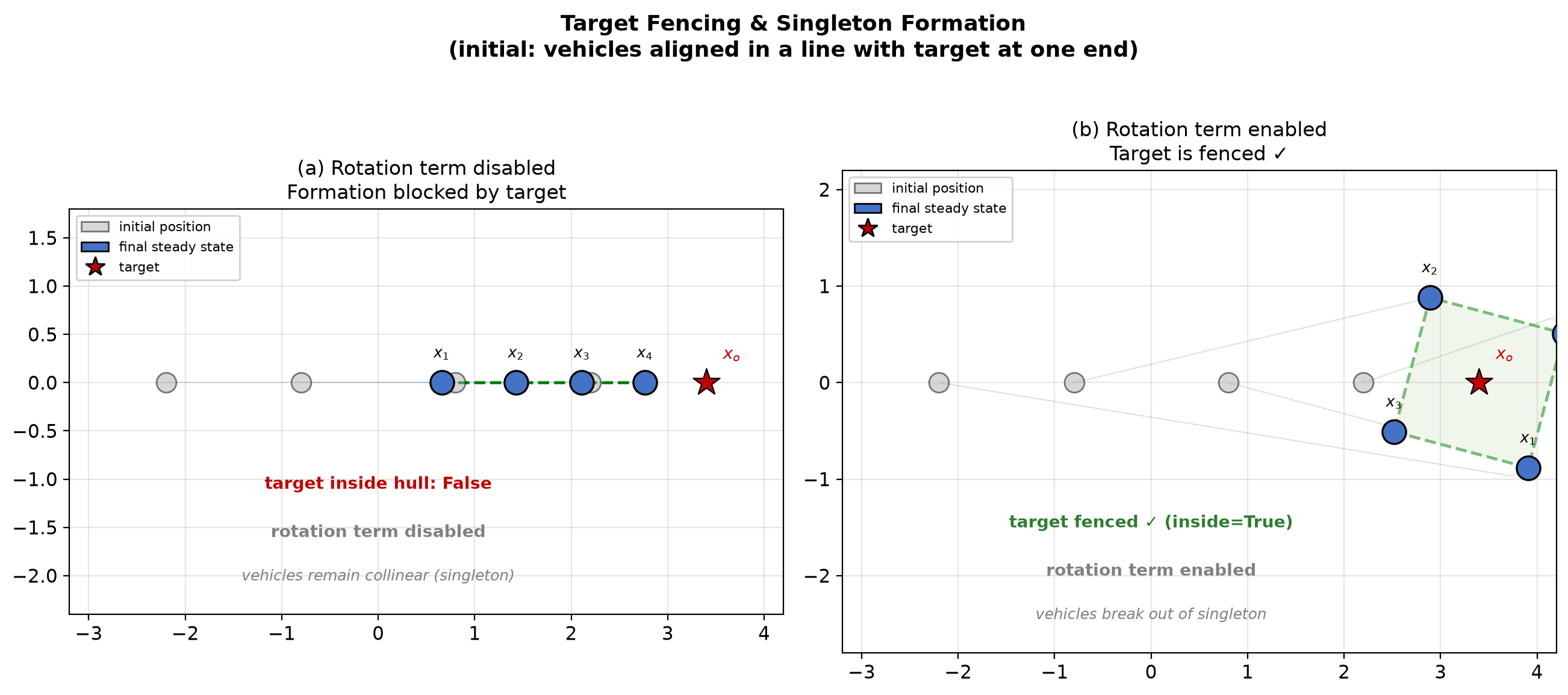
Consider the case where vehicles are aligned in a straight line with the target at one end.
Using the modified controller

the target will be fenced — provided the rotation term is active.

If the rotation term is disabled, the vehicles remain collinear and the formation is blocked by the target (the target stays at one end of the line, outside the convex hull).

4.2 Obstacle collision avoidance#

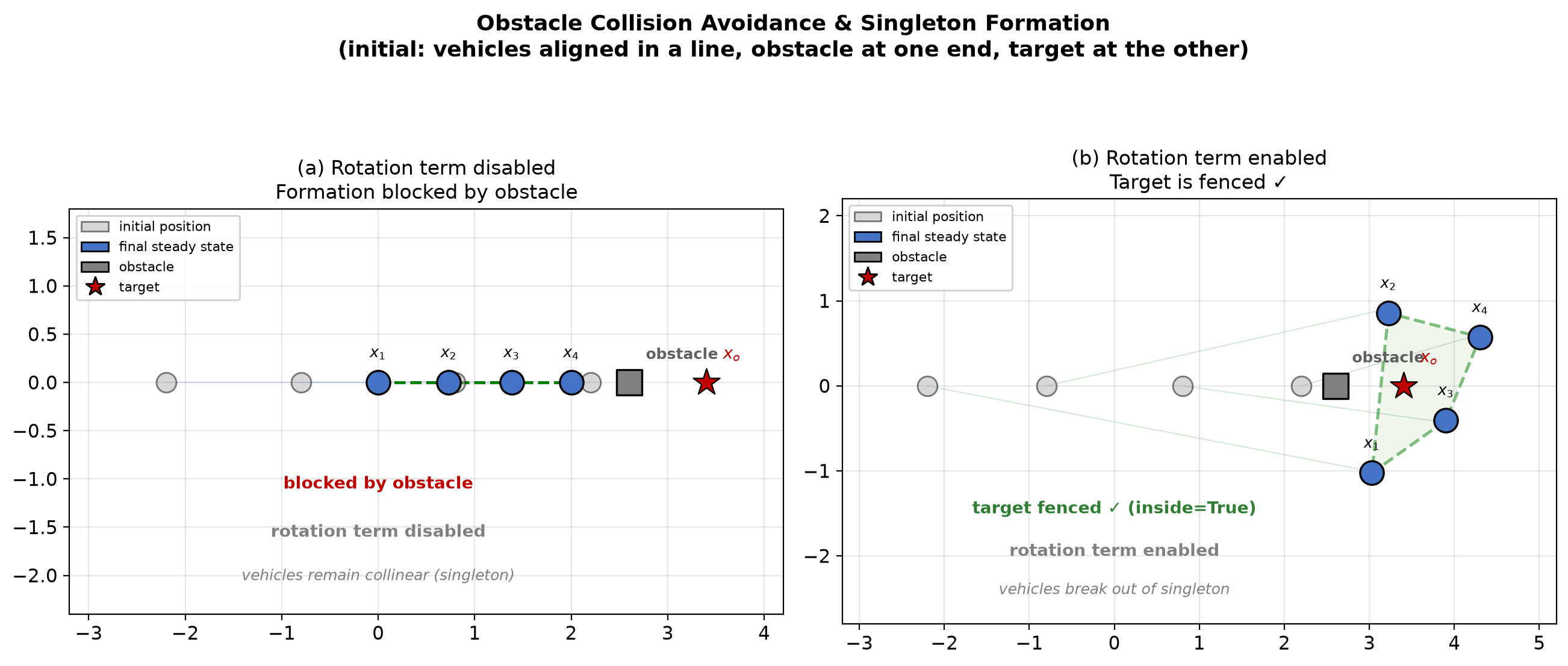
Consider the case where vehicles are aligned in a straight line with the target and one point obstacle. The obstacle and the target are positioned at one end of the line.
Using the modified controller

the target will be fenced provided the rotation term is active. Otherwise, the formation will be blocked by the obstacle.

4.3 Drawback of the rotation term#

The paper proves that no collision occurs for $t \in [0, \infty)$, but asymptotic collision ($t \to \infty$) is not ruled out.
This is mainly due to the residual term $\psi_i$ in inequality (*), which is difficult to analyse precisely.

In practice, this drawback is not a serious concern, since $t \to \infty$ may not exist in the physical world.