Bifurcations in fencing control (Kou et al. 2021 TAC algorithm 1)

Most existing results on flocking/fencing control achieve the velocity‑matching property, which is typically guaranteed via a Lyapunov function. However, the first algorithm presented in (Kou et al. 2021 TAC algorithm 1)¹ only guarantees that the average velocity of all agents converges to the target value. The final formation yielded by this algorithm exhibits several intriguing phenomena, which I suspect may correspond to bifurcations.

Controller#

The controller only consists of there terms: target attraction, neighbor repulsion and integral of target attraction.

\begin{aligned} \dot{p}_i=u_i &= \varphi_i + k_1(x_0 - x_i) + v_i \\ \dot{v}_i &= k_2(x_0 - x_i) \end{aligned}

Here, the central repulsion function is selected as $\alpha(s) = 1/(s-d) - 1/(\mu-d)$ for $s \in (d, \mu]$ . The paper proved that the target with constant speed can be fenced with this controller. Different from other fencing results, the final formation will rotate about the target as demonstrated in its paper.

Three regimes#

	1D	2D rigid rotation	2D breathing
$N$	5	6	5
$d / \mu$	$0.5 / 2.0$	$5.0 / 9.0$	$5.0 / 9.0$
$k_1 / k_2$	$1.0 / -$	$0.5 / 0.5$	$0.5 / 0.5$
$v_0$	$1.0$	$(1, 0)$	$(1, 0)$
Behavior	Static equilibrium in target frame	$\\|\omega\\| = \sqrt{k_2}$	$T \approx 2.49\text{s}$ , $\omega_\text{eff}/\sqrt{k_2} \approx 3.57$

1D#

x_0 = [-0.75, 2.70, 1.39, 0.59, -2.06]

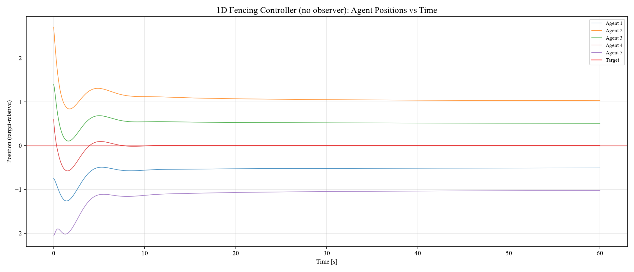
Vehicles converge to a static formation that fences the target. Velocity error $\to 0$ . The space between two nearby vehicles converges to the minimum safety distance $d$ .

2D rigid rotation#

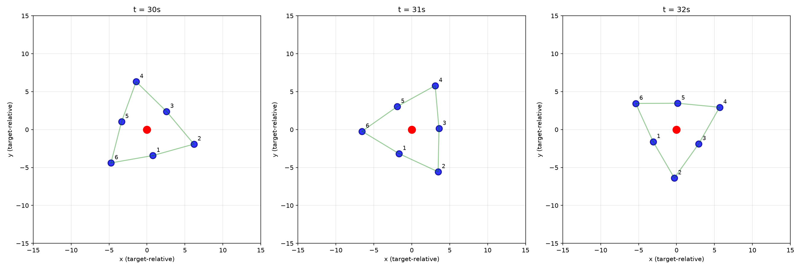
x_0 = \textrm{regular hexagon}, R = 8.0 \quad v_0 = [1, 0]^T

Formation rotates at $|\omega| = \sqrt{k_2} = 0.707$ which can be verified with analysis.

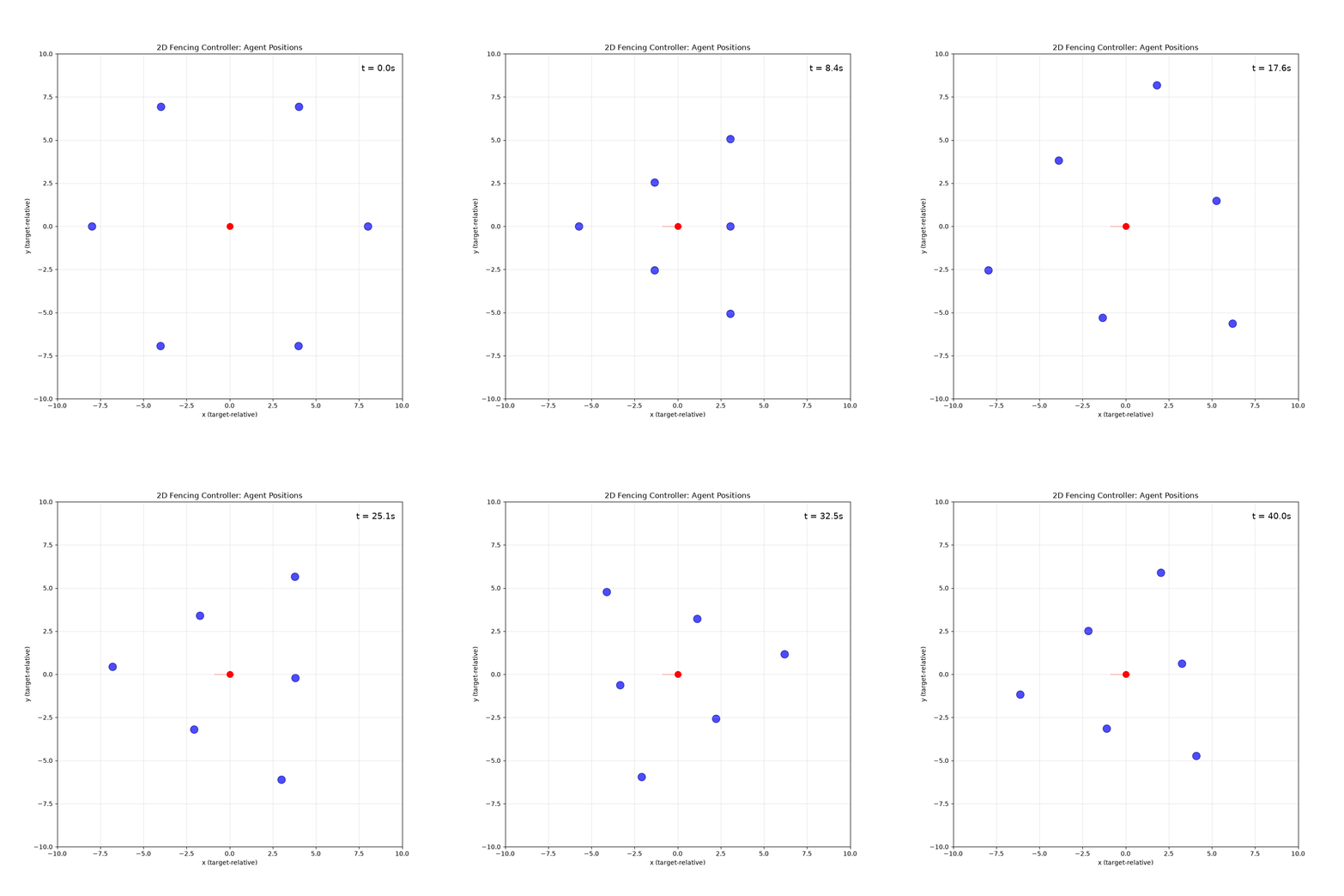
Steady-state snapshots at $t = 30, 31, 32$ s:

2D breathing limit cycle#

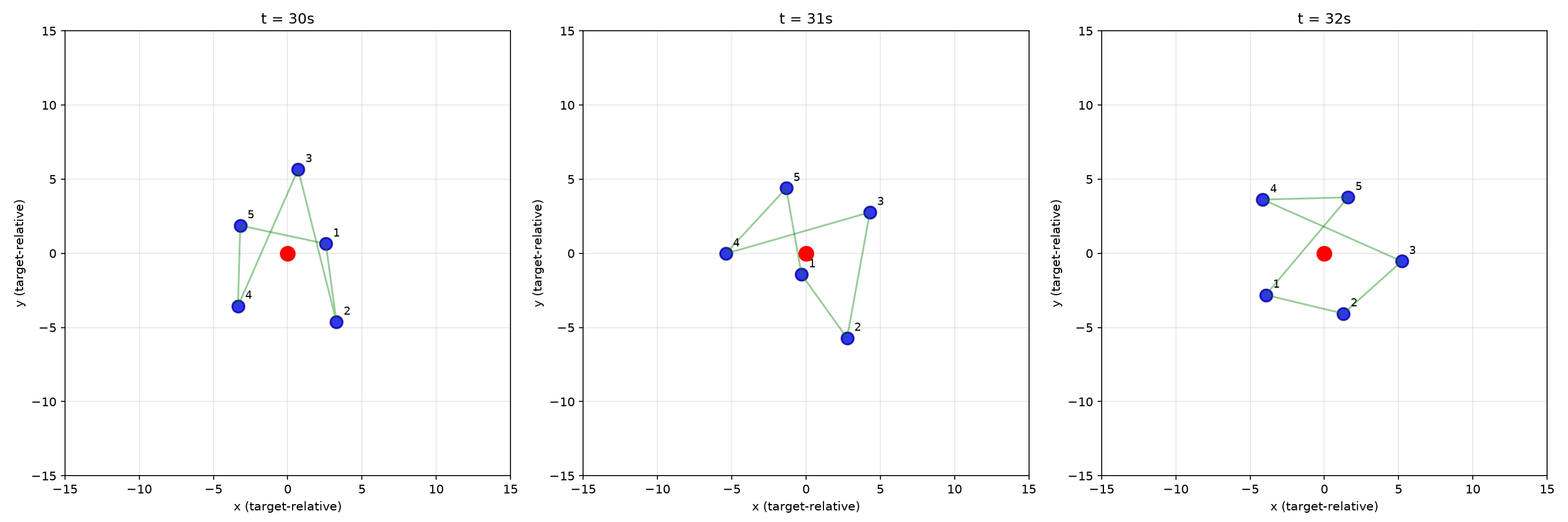
x_0 = [[-10.58, -12.53], [-5.38, 5.90], [-0.18, 9.18], [-7.35, -4.81], [-6.29, 12.44]] \quad v_0 = [1, 0]^T

Non-symmetric initial conditions. Pairwise distances oscillate periodically — the formation breathes instead of rotating rigidly.

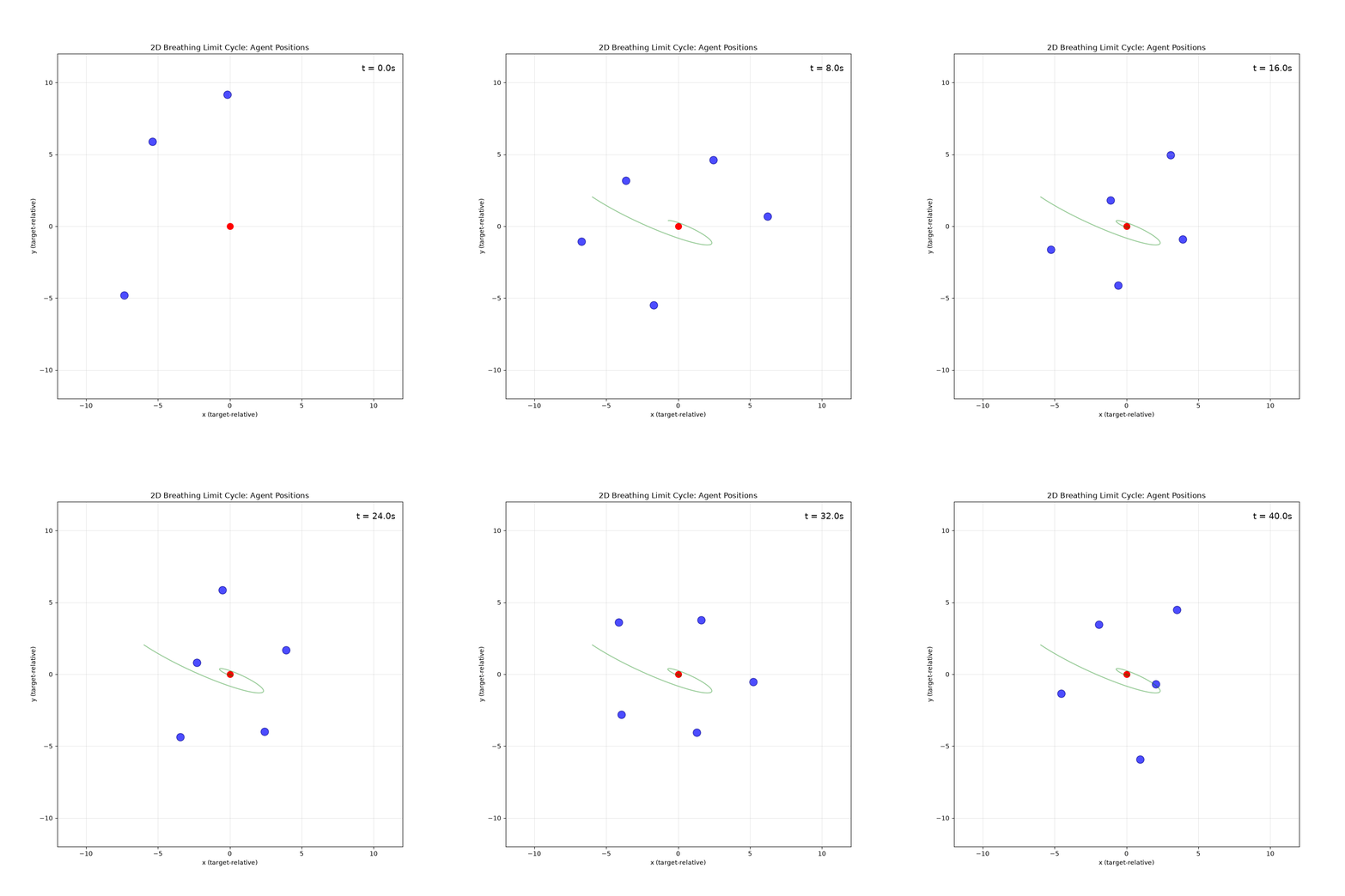
Steady-state snapshots at $t = 30, 31, 32$ s:

3D non-planar rotation#

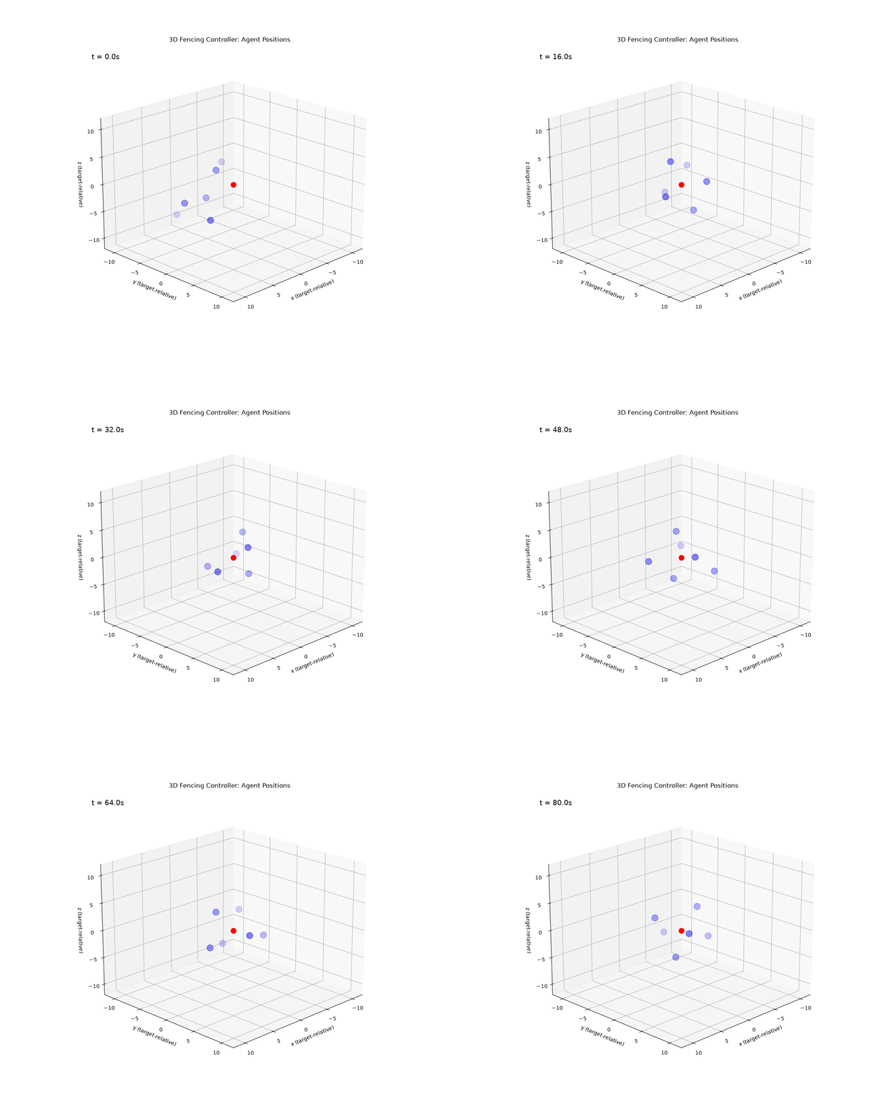
x_0 = \textrm{random 3D positions}\quad v_0 = (1, 0, 0)

With random 3D initial conditions, vehicles form a genuinely non-planar rotating formation ( $\sigma_3/\sigma_1 \approx 0.91$ ). Planar initial conditions stay planar — confirming the code is correct and the 3D behavior is real.

Key insight#

The controller constrains only the average position error and average velocity, leaving $2(N-1)$ circulation degrees of freedom unconstrained. Different initial conditions excite different attractors: rigid rotation, breathing limit cycle, or 3D non-planar orbits.

Is it possible for this system to be a chaos system?

L. Kou, Z. Chen and J. Xiang, “Cooperative Fencing Control of Multiple Vehicles for a Moving Target With an Unknown Velocity,” in IEEE Transactions on Automatic Control, vol. 67, no. 2, pp. 1008-1015, Feb. 2022, doi: 10.1109/TAC.2021.3075320. ↩︎